What do physicists do? I have been thinking a bit about what I do and what the true job of a physicist is and I think I can state it as finding the fundamental variables that most appropriately describe a physical problem. Usually, once these so-called "degrees-of-freedom" are found, the problem is solved.
Sounds easy enough, however, Nature can be tricky. The degrees of freedom that we call "fundamental" in one setting may not be the same in a slightly different setting. What may be important to describe the system under some conditions may not be so under different conditions; which poses the question: How do you transform one set of degrees of freedom into another? Telling these situations apart and learning how to "combine" one set into another is quite complicated. Essentially, we need to have a deeper understanding of our theories, well beyond the one used in daily applications and technology. That is, we need to sharpen our ability to go beyond approximations and stable situations, moving towards conclusions which acknowledge the system as a whole more completely. It is not enough, anymore, to only look at bits and pieces and try and infer the behavior of the whole system.
Which brings me to the topic of phase transitions. Phase transitions are well understood classically (the whole topic is called "thermodynamics") but not so much so quantum mechanically. But something has been brewing for quite some time, and has now found its way into more glorious pastures: Quantum Phases--something that FQXi researcher Subir Sachdev has been looking into (see the article "The Black Hole and the Babel Fish" for more details) and which has caught the attention of the media recently because it uses string theory techniques to explain condensed matter phenomena. I have been working on a related area at Syracuse University. Of course, this is a project still in its speculatory infancy. But, there are some positive and encouraging results and I will outline these here.
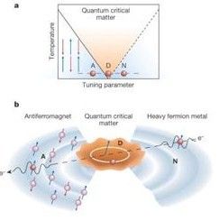
In condensed matter physics, quantum phases are defined to be the different quantum states at zero temperature. A quantum phase transition (QPT) happens when a system undergoes a change from one quantum phase to another, at zero temperature. It describes an abrupt change in the ground-state of the system caused by its quantum fluctuations. A quantum critical point (QCP) is a point in the phase diagram of a system (at zero temperature) that separates two quantum phases. (The image above is taken from Piers Coleman and Andrew J. Schofield, Nature 433, 226-229, shows the phase diagram (a) and the growth of droplets of quantum critical matter near the quantum critical point (b).)
In addition to this, QCPs distort the fabric of the phase diagram creating a phase of "quantum critical matter" fanning out to finite temperatures from the QCP. In an analogy with a Black Hole, no information about the microscopic nature of the system affects the quantum critical matter, that is, the passage from a non-critical to a critical quantum phase requires crossing an "event horizon". As expected, at the QCP, the system exhibits spacetime scale invariance, justifying the idea that it can be modeled via a Conformal Field Theory (CFT)--because of this, sometimes the QCP is referred only as a "conformal point" of the system.
At this point, we are almost ready to make a connection with high energy physics, namely with quantum field theory (QFT), but to set the stage, let us start with an example: an ultralocal spin 0 bosonic field, also known as a scalar field in 0-dimensions, which I'll give the following potential:
[equation]$V(\phi) = \frac{\mu}{2}\, \phi^{2} \frac{\lambda}{4}\, \phi^{4} \;.$[/equation]
All of the desired objects in this little example are well defined: Path Integral (aka, Partition Function), Schwinger-Dyson equations, Fourier Transforms, etc.
The Partition Function is given by, [equation]$ \mathcal{Z}[\mu, \lambda ;\, J] = \int_{\Gamma} e^{i\, (\frac{\mu}{2}\, \phi^{2} \frac{\lambda}{4}\, \phi^{4}) - i\, J\, \phi}\, \mathrm{d}\phi \; ; $[/equation]
where Γ is the integration region (or integration contour, as I'll explain shortly), while the Schwinger-Dyson equation is:
[equation]$ (\lambda\, \partial^3_J \mu\, \partial_J)\, \mathcal{Z} = J $[/equation]
where we have used [equation]\phi \mapsto -i\, \partial_J .[/equation]
The only meaningful parameter in this problem is a combination of both coupling constants, namely [equation]$ g = \mu/\lambda $[/equation] and [equation]$ \lambda \neq 0. $[/equation]
The Schwinger-Dyson equation and the Partition Function are just two expressions of the same problem. So, given that we have a 3rd order differential equation, we must have 3 different solutions. Which brings me back to the integration contour Γ above: we must have 3 distinct contours in order to find all possible solutions to our problem. Note that we can Fourier Transform the Schwinger-Dyson equation above and obtain a polynomial equation, with complex-valued solutions labelled by g.
[equation]p^3 g\, p = 0 \; .[/equation]
So, the bottom line is this little quantum toy model of ours has three different solutions, i.e., its moduli space has three points.
The three solutions of the differential equation above (Schwinger-Dyson) are called Parabolic Cylinder Functions, [equation]U(g,J),\, V(g,J),\, W(g,J),[/equation] all dependent on g.
Let us make some straightforward observations. We needed three different boundary conditions (i.e., D-branes) to find all possible solutions to the Schwinger-Dyson equations, which is analogous to saying that we needed three different contours [equation]$ \Gamma_1,\, \Gamma_2,\, \Gamma_3 $[/equation] in order to appropriately define the Partition Function. More explicitly, we have three different Partition Functions, all originating from the same toy model, with three different "quantum systems" as solutions, where each system is determined by the allowed values of g. Furthermore, each one of these allowed ranges of g corresponds to a point in the moduli space of the polynomial equation we found above.
We can now try and adopt a dynamical systems viewpoint. Essentially, in a graph of [equation]$ \partial\phi = \pi, $[/equation] we would get three attractors whose basins and flows are not trivial. (The image, right, is a visual aid showing attractors, taken from Wikipedia, but it's not directly related to the construction mentioned here.) If we playing with the values of g inside each of the three distinct ranges, these flows and basins vary smoothly; however, when the values get closer and closer to the boundaries of the different ranges, we start to see the appearance of "folds," "cusps," and "catastrophes". This is equivalent to studying the singularities of the polynomial we found above; which is also analogous to finding the singular points formed in the level sets of the Potential function. At the same time, the Schwinger-Dyson equations for these different values of the parameter g, undergo Stokes phenomena along lines of accumulation of Lee-Yang zeros, which creates regions of analyticity for the Partition Function.
At this point, we are ready for the punchline: Each inequivalent vacua of this toy model of ours, delimited by the equivalence class of the allowed values of g, corresponds to a different quantum phase. After all, each quantum phase is nothing but the ground state of the model. Indeed, each of the parabolic cylinder functions above has a very distinct behavior, defining vacuum states that have quite different properties. In fact, the asymptotic expansion of each of these functions yields very different behavior: one is amenable to perturbation theory (i.e., coupling constant expansion, known as the symmetric phase); the other one behaves like a soliton; and the last one is known as the broken-symmetric phase.
To be continued in my next post. Stay tuned.